Quickstart#
Show code cell content
%config InlineBackend.figure_format = "png"

from matplotlib import rcParams

rcParams["savefig.dpi"] = 100
rcParams["figure.dpi"] = 300

rcParams["font.family"] = "serif"
rcParams["mathtext.fontset"] = "dejavuserif"
To get you started, here’s an annotated, fully-functional example that demonstrates the usage of pyLick using a spectrum of an individual galaxy taken from the LEGA-C DR3 survey (data from the ESO portal; data release paper: van der Wel et al., 2021).
The first thing that we need to do is to import the necessary modules:
osandpylick.ioto deal with data I/O,numpyto perform spectrum manipulation,the
Galaxyclass to measure spectral indices.
import os
import numpy as np
import pylick.io as io
import pylick.plot as plot
from pylick.analysis import Galaxy
Then, we create a folder and download a LEGA-C DR3 (van de Wel et al. 2021) spectrum from the ESO archive.
dir_data = os.path.dirname(io.__file__) + "/../docs/tutorials/data/"

# Test with different galaxies!
k = 2

if k==0:
    # ID M10_213772
    filename = "legac_M10_213772_v3.0.fits"
    os.system("wget https://dataportal.eso.org/dataportal_new/file/ADP.2021-07-29T07:33:58.941 -P {:s} >/dev/null 2>&1".format(dir_data))
    os.system("mv {:s}/ADP.2021-07-29T07:33:58.941 {:s}/{:s}".format(dir_data,dir_data,filename))
    z = 0.6999

elif k==1:
    # ID M11_217260
    filename = "legac_M11_217260_v3.0.fits"
    os.system("wget https://dataportal.eso.org/dataportal_new/file/ADP.2021-07-29T07:33:59.128 -P {:s} >/dev/null 2>&1".format(dir_data))
    os.system("mv {:s}/ADP.2021-07-29T07:33:59.128 {:s}/{:s}".format(dir_data,dir_data,filename))
    z = 0.6987

elif k==2:
    # ID M2_132048
    filename = "legac_M2_132048_v3.0.fits"
    os.system("wget https://dataportal.eso.org/dataportal_new/file/ADP.2021-07-29T07:34:01.368 -P {:s} >/dev/null 2>&1".format(dir_data))
    os.system("mv {:s}/ADP.2021-07-29T07:34:01.368 {:s}/{:s}".format(dir_data,dir_data,filename))
    z= 0.6686
We load the .fits spectrum by using the io.load_spec_fits() function. The spectrum is assumed to be (and usually it is) at the 1st extension of the Header Data Unit (HDU), this can be changed by passing, e.g. hdul=0. We then pass the column names for the data that we want to extract (in this case the wavelenght sampling, flux, flux uncertainties, and the pixels’ quality flag). We may also want to mask out the side regions where the flux is equal to 0 by setting reduce_window=True.
We mask bad pixels (flagged or flux equal to 0) and call io.spec_stats() in the final spectrum arrays: this is useful to check if there are some problems with the spectrum before measuring indices on it!
colnames = ['wave', 'flux', 'err', 'qual']
spec_raw = io.load_spec_fits(dir_spec=dir_data, filename=filename, colnames=colnames, reduce_window=False, hdul=1)

# Mask bad pixels and ferr==0 pixels
bad_pixels       = np.logical_or(spec_raw[3]==1,spec_raw[2]==0)
wave, flux, ferr = [spec_raw[i][~bad_pixels] for i in [0,1,2]]

# Quick look
io.spec_stats(wave, flux, ferr)
 wave)	 range: 6060.1--8500.3	 mean: 7274.02	 median: 7277.8
 flux)	 range: 80.41--410.43	 mean: 276.14	 median: 302.73
 ferr)	 range: 1.74--9.12	 mean: 2.33	 median: 2.08
 delta_wave_mean: 0.64
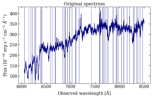
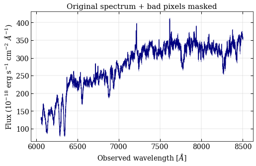
Let’s have a quick look at the spectrum. First of all the raw version, where bad pixels have been assigned a flux error of 9e9 (producing the vertical lines). Then, the cleaned version, where bad pixels are removed. The code can handle both cases, but in the first one it will be possible to retrieve the bad/total pixel fraction inside each measured index.
plot_raw   = plot.spectrum_simple(spec_raw[0], spec_raw[1], spec_raw[2], mask=bad_pixels)
plot_clean = plot.spectrum_simple(wave, flux, ferr)

plot_raw.gca().set_title("Original spectrum", fontsize=15)
plot_raw.gca().set_ylabel(r"Flux (10$^{-18}$ erg s$^{-1}$ cm$^{-2}$ $\AA^{-1}$)")
plot_raw.gca().set_xlabel(r"Observed wavelength [$\AA$]")

plot_clean.gca().set_title("Original spectrum + bad pixels masked", fontsize=15)
plot_clean.gca().set_ylabel(r"Flux (10$^{-18}$ erg s$^{-1}$ cm$^{-2}$ $\AA^{-1}$)")
plot_clean.gca().set_xlabel(r"Observed wavelength [$\AA$]")

plot_clean.gca().grid(color="silver", lw=.4)
Optional. By importing the IndexLibrary class, we can have a first look at the available indices and their keys to be passed to pyLick. The full library of the available indices can be retrieved by setting keys=None. In the documentation, we also provide a separate tutorial on how to define and measure a new set of spectral indices with pyLick.
from pylick.indices import IndexLibrary

index_keys = np.arange(22, 47)
lib        = IndexLibrary(index_keys=index_keys)

print(lib)
ID  name     unit      blue               centr              red                tex_name
-------------------------------------------------------------------------------------------
22  CaII_K   A         3845.000-3880.000  3925.650-3945.000  3950.000-3954.000  CaII~K
23  CaII_H   A         3950.000-3954.000  3959.400-3975.000  3983.000-3993.000  CaII~H
24  D4000    break_nu  3750.000-3950.000     0.000-   0.000  4050.000-4250.000  D4000
25  Dn4000   break_nu  3850.000-3950.000     0.000-   0.000  4000.000-4100.000  D_{n}4000
26  Hdelta_A A         4041.600-4079.750  4083.500-4122.250  4128.500-4161.000  H\delta_A
27  Hdelta_F A         4057.250-4088.500  4091.000-4112.250  4114.750-4137.250  H\delta_F
28  CN1      mag       4080.125-4117.625  4142.125-4177.125  4244.125-4284.125  CN_1
29  CN2      mag       4083.875-4096.375  4142.125-4177.125  4244.125-4284.125  CN_2
30  Ca4227   A         4211.000-4219.750  4222.250-4234.750  4241.000-4251.000  Ca4227
31  G4300    A         4266.375-4282.625  4281.375-4316.375  4318.875-4335.125  G4300
32  Hgamma_A A         4283.500-4319.750  4319.750-4363.500  4367.250-4419.750  H\gamma_A
33  Hgamma_F A         4283.500-4319.750  4331.250-4352.250  4354.750-4384.750  H\gamma_F
34  Fe4383   A         4359.125-4370.375  4369.125-4420.375  4442.875-4455.375  Fe4383
35  Ca4455   A         4445.875-4454.625  4452.125-4474.625  4477.125-4492.125  Ca4455
36  Fe4531   A         4504.250-4514.250  4514.250-4559.250  4560.500-4579.250  Fe4531
37  C2_4668  A         4611.500-4630.250  4634.000-4720.250  4742.750-4756.500  C_{2}4668
38  Hbeta    A         4827.875-4847.875  4847.875-4876.625  4876.625-4891.625  H_\beta
39  Fe5015   A         4946.500-4977.750  4977.750-5054.000  5054.000-5065.250  Fe5015
40  Mg1      mag       4895.125-4957.625  5069.125-5134.125  5301.125-5366.125  Mg_1
41  Mg2      mag       4895.125-4957.625  5154.125-5196.625  5301.125-5366.125  Mg_2
42  Mgb      A         5142.625-5161.375  5160.125-5192.625  5191.375-5206.375  Mg_b
43  Fe5270   A         5233.150-5248.150  5245.650-5285.650  5285.650-5318.150  Fe5270
44  Fe5335   A         5304.625-5315.875  5312.125-5352.125  5353.375-5363.375  Fe5335
45  Fe5406   A         5376.250-5387.500  5387.500-5415.000  5415.000-5425.000  Fe5406
46  Fe5709   A         5672.875-5696.625  5696.625-5720.375  5722.875-5736.625  Fe5709
Now pyLick can work for us! Note that if z is not passed, the spectrum is assumed to be already rest frame.
index_keys = np.arange(22, 47)
indices    = Galaxy(filename, index_keys,
                    wave=wave, flux=flux, ferr=ferr,
                    mask=None, meas_method='int', z=z, plot=True)

print(indices)
> Index outside of the spectrum (3631.85 < lambda < 5094.27)
> Index outside of the spectrum (3631.85 < lambda < 5094.27)
> Index outside of the spectrum (3631.85 < lambda < 5094.27)
> Index outside of the spectrum (3631.85 < lambda < 5094.27)
> Index outside of the spectrum (3631.85 < lambda < 5094.27)
> Index outside of the spectrum (3631.85 < lambda < 5094.27)
> Index outside of the spectrum (3631.85 < lambda < 5094.27)
Elapsed time: 0.01 s

names           vals       errs
---------------------------------
CaII_K         2.0039     0.0458
CaII_H        -0.0235     0.0317
D4000          1.4795     0.0008
Dn4000         1.1666     0.0009
Hdelta_A       1.3758     0.0379
Hdelta_F      -0.7634     0.0293
CN1            0.0564     0.0011
CN2            0.0703     0.0012
Ca4227        -0.1843     0.0199
G4300         -0.4446     0.0337
Hgamma_A       0.7180     0.0341
Hgamma_F       1.1900     0.0215
Fe4383        -1.0463     0.0589
Ca4455        -0.1048     0.0290
Fe4531        -0.9484     0.0545
C2_4668        5.9379     0.0801
Hbeta          0.1699     0.0309
Fe5015        -2.0909     0.0886
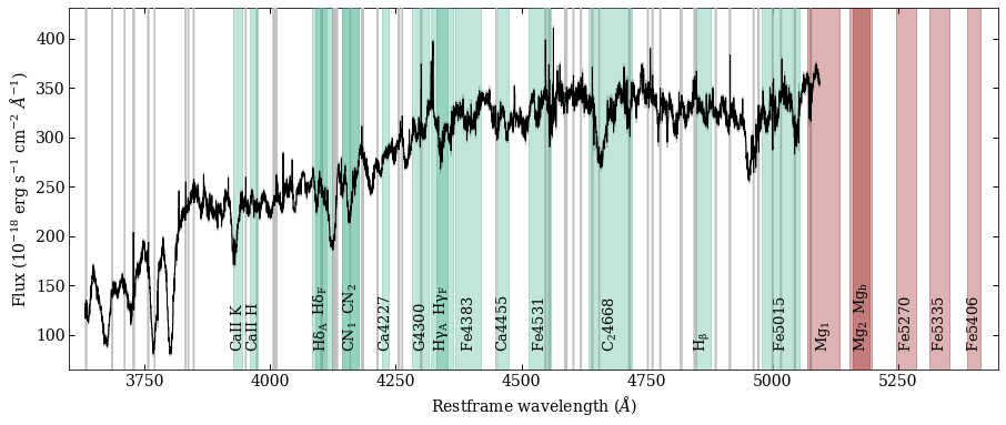
Finally, we plot the spectrum with the measured indices. In the following cell, we do it manually by calling variables defined previously. However it can be automatically saved when calling the Galaxy class by setting the parameter plot=True.
plot_spec = plot.spectrum_with_indices(wave, flux, ferr=ferr,
                                       index_regions=lib.regions,
                                       index_names=lib.tex_names,
                                       index_units=lib.units,
                                       z=z, mask=None, ax=None,
                                       index_done=None,
                                       settings={'figsize': (15,6)})
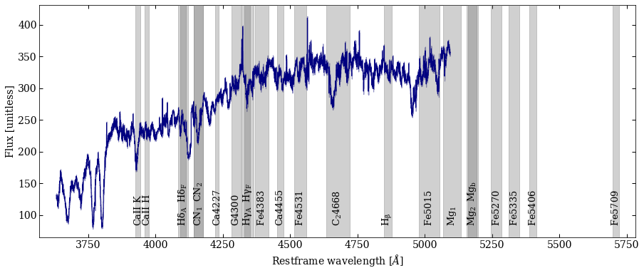
The plot can be further modified. To display only the mesured indices we can pass a boolean mask using index_done, while if set settings['inspect']=True non-measured indices will be displayed in red. We can also change other properties using the settings dictionary. In this last plot we will display the original (raw) spectrum and its bad pixels.
index_done    = np.isfinite(indices.vals)
user_plParams = {'figsize': (15,6),
                'xlab': r"Restframe wavelength ($\AA$)",
                'ylab': r"Flux (10$^{-18}$ erg s$^{-1}$ cm$^{-2}$ $\AA^{-1}$)",
                # Colors of: flux, ferr, indices
                'spec_colors': ['k', 'silver', '#33A980'],
                # Fontsizes of: title, labels, indices
                'spec_fontsizes': [14, 14, 13],
                'format': '.pdf',
                # Debug
                'inspect': True,
                }

plot_spec = plot.spectrum_with_indices(spec_raw[0], spec_raw[1], ferr=spec_raw[2],
                                       index_regions=lib.regions,
                                       index_names=lib.tex_names,
                                       index_units=lib.units,
                                       z=z, mask=bad_pixels, ax=None,
                                       index_done=index_done,
                                       settings=user_plParams)
plot_spec.gca().set_xlim(3600, 5450)
(3600.0, 5450.0)